Xarray accessors
One of the main purposes of Salem is to add georeferencing tools to
xarray ‘s data structures. These tools can be accessed via a special
.salem attribute, available for both xarray.DataArray and
xarray.Dataset objects after a simple import salem in your code.
Initializing the accessor
Automated projection parsing
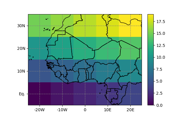
Salem will try to understand in which projection your Dataset or DataArray is defined. For example, with a platte carree (or lon/lat) projection, Salem will know what to do based on the coordinates’ names:
In [1]: import numpy as np

In [2]: import xarray as xr

In [3]: import salem

In [4]: da = xr.DataArray(np.arange(20).reshape(4, 5), dims=['lat', 'lon'],
   ...:                   coords={'lat':np.linspace(0, 30, 4),
   ...:                           'lon':np.linspace(-20, 20, 5)})
   ...:

In [5]: da.salem  # the accessor is an object
Out[5]: <salem.sio.DataArrayAccessor at 0x7f9773522210>

In [6]: da.salem.quick_map();
While the above should work with a majority of climate datasets (such as atmospheric reanalyses or GCM output), certain NetCDF files will have a more exotic map projection requiring a dedicated parsing. There are conventions to formalise these things in the NetCDF data model, but Salem doesn’t understand them yet (my impression is that they aren’t widely used anyways).
Currently, Salem can deal with:
platte carree (or lon/lat) projections
WRF projections (see WRF tools)
for geotiff files only: any projection that rasterio can understand
virually any projection provided explicitly by the user
The logic for deciding upon the projection of a Dataset or DataArray is
located in grid_from_dataset(). If the automated parsing
doesn’t work, the salem accessor won’t work either. In that case, you’ll
have to provide your own Custom projection to the data.
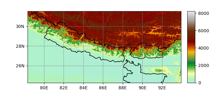
From geotiffs
Salem uses rasterio to open and parse geotiff files:
In [7]: fpath = salem.get_demo_file('himalaya.tif')

In [8]: ds = salem.open_xr_dataset(fpath)

In [9]: hmap = ds.salem.get_map(cmap='topo')

In [10]: hmap.set_data(ds['data'])

In [11]: hmap.visualize();
Custom projection
Alternatively, Salem will understand any projection supported by pyproj. The proj info has to be provided as attribute:
In [12]: dutm = xr.DataArray(np.arange(20).reshape(4, 5), dims=['y', 'x'],
   ....:                     coords={'y': np.arange(3, 7)*2e5,
   ....:                             'x': np.arange(1, 6)*2e5})
   ....:

In [13]: psrs = 'epsg:32630'  # http://spatialreference.org/ref/epsg/wgs-84-utm-zone-30n/

In [14]: dutm.attrs['pyproj_srs'] = psrs

In [15]: dutm.salem.quick_map(interp='linear');
Using the accessor
The accessor’s methods are available trough the .salem attribute.
Keeping track of attributes
Some datasets carry their georeferencing information in global attributes (WRF
model output files for example). This makes it possible for Salem to
determine the data’s map projection. From the variables alone,
however, this is not possible. This is the reason why it is recommended to
use the open_xr_dataset() and
open_wrf_dataset() function, which add
an attribute to the variables automatically:
In [16]: dsw = salem.open_xr_dataset(salem.get_demo_file('wrfout_d01.nc'))

In [17]: dsw.T2.pyproj_srs
Out[17]: '+proj=lcc +lat_0=29.0399971008301 +lon_0=89.8000030517578 +lat_1=29.0400009155273 +lat_2=29.0400009155273 +x_0=0 +y_0=0 +R=6370000 +units=m +no_defs'
Unfortunately, the DataArray attributes are lost when doing operations on them. It is the task of the user to keep track of this attribute:
In [18]: dsw.T2.mean(dim='Time', keep_attrs=True).salem  # triggers an error without keep_attrs
Out[18]: <salem.sio.DataArrayAccessor at 0x7f9773bd15e0>
Reprojecting data
You can reproject a Dataset onto another one with the
transform() function:
In [19]: dse = salem.open_xr_dataset(salem.get_demo_file('era_interim_tibet.nc'))
In [20]: dsr = ds.salem.transform(dse)
In [21]: dsr
Out[21]:
<xarray.Dataset>
Dimensions: (time: 4, x: 1875, y: 877)
Coordinates:
* time (time) datetime64[ns] 2012-06-01 ... 2012-06-01T18:00:00
* x (x) float64 78.32 78.33 78.34 78.35 ... 93.91 93.92 93.93 93.94
* y (y) float64 31.54 31.53 31.52 31.51 ... 24.26 24.25 24.25 24.24
Data variables:
t2m (time, y, x) float64 278.6 278.6 278.6 278.6 ... 296.2 296.2 296.2
Attributes:
pyproj_srs: +proj=longlat +datum=WGS84 +no_defs
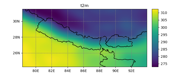
In [22]: dsr.t2m.mean(dim='time').salem.quick_map();

Currently, salem implements, the neirest neighbor (default), linear, and spline interpolation methods:
In [23]: dsr = ds.salem.transform(dse, interp='spline')

In [24]: dsr.t2m.mean(dim='time').salem.quick_map();
The accessor’s map transformation machinery is handled by the
Grid class internally. See Map transformations for more information.
Subsetting data
The subset() function allows you to subset
your datasets according to (georeferenced) vector or raster data, for example
based on shapely geometries
(e.g. polygons), other grids, or shapefiles:
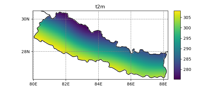
In [25]: shdf = salem.read_shapefile(salem.get_demo_file('world_borders.shp'))
In [26]: shdf = shdf.loc[shdf['CNTRY_NAME'] == 'Nepal'] # remove other countries
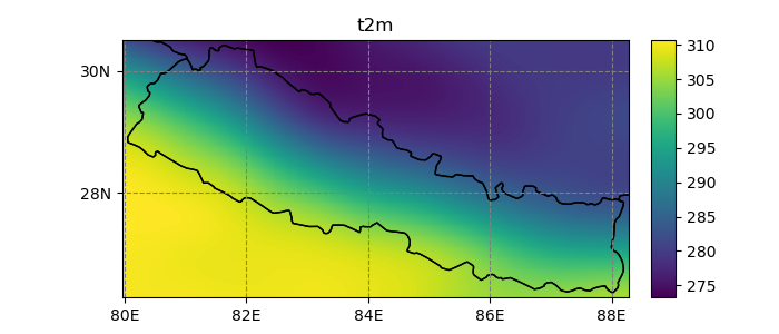
In [27]: dsr = dsr.salem.subset(shape=shdf, margin=10)
In [28]: dsr.t2m.mean(dim='time').salem.quick_map();
Regions of interest
While subsetting selects the optimal rectangle over your region of interest,
sometimes you also want to maskout unrelevant data, too. This is done with the
roi() tool:
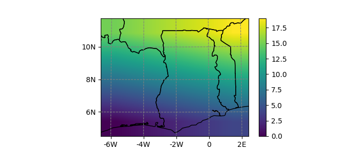
In [29]: dsr = dsr.salem.roi(shape=shdf)

In [30]: dsr.t2m.mean(dim='time').salem.quick_map();