xarray accessors¶

One of the main purposes of Salem is to add georeferencing tools to xarray ‘s data structures. These tools can be accessed via a special .salem attribute, available for both xarray.DataArray and xarray.Dataset objects after a simple import salem in your code.

Initializing the accessor¶

Automated projection parsing¶

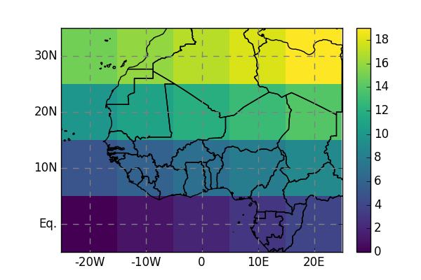
Salem will try to understand in which projection the Dataset or DataArray is defined. For example, with a platte carree (or lon/lat) projection, Salem will know what to do based on the coordinates’ names:

In [1]: import numpy as np

In [2]: import xarray as xr

In [3]: import salem

In [4]: da = xr.DataArray(np.arange(20).reshape(4, 5), dims=['lat', 'lon'],
   ...:                   coords={'lat':np.linspace(0, 30, 4), 'lon':np.linspace(-20, 20, 5)})
   ...: 

In [5]: da.salem
Out[5]: <salem.sio.DataArrayAccessor at 0x7fd3c0c93f10>

In [6]: da.salem.quick_map();

While the above should work with many (most?) climate datasets (such as atmospheric reanalyses or GCM output), certain NetCDF files will have a less standard map projection requiring special parsing. There are conventions to formalise these things in the NetCDF model, but Salem doesn’t understand them yet. Currently, Salem can parse: - platte carree (or lon/lat) projections - WRF projections (see WRF tools) - virually any projection explicitly provided by the user - for geotiff files only: any projection that rasterio can understand

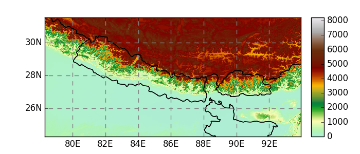
From geotiffs¶

Salem uses rasterio to open and parse geotiff files:

In [7]: fpath = salem.get_demo_file('himalaya.tif')

In [8]: ds = salem.open_xr_dataset(fpath)

In [9]: hmap = ds.salem.get_map(cmap='topo')

In [10]: hmap.set_data(ds['data'])

In [11]: hmap.visualize();

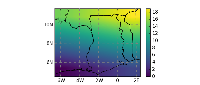
Custom projections¶

Alternatively, Salem will understand any projection supported by pyproj. The proj info has to be provided as attribute:

In [12]: dutm = xr.DataArray(np.arange(20).reshape(4, 5), dims=['y', 'x'],
   ....:                     coords={'y': np.arange(3, 7)*2e5,
   ....:                             'x': np.arange(1, 6)*2e5})
   ....: 

In [13]: psrs = 'epsg:32630'  # http://spatialreference.org/ref/epsg/wgs-84-utm-zone-30n/

In [14]: dutm.attrs['pyproj_srs'] = psrs

In [15]: dutm.salem.quick_map(interp='linear');

Using the accessor¶

The accessor’s methods are available trough the .salem attribute.

Keeping track of attributes¶

Some datasets carry their georeferencing information in global attributes (WRF model output files for example). This makes it possible for Salem to determine the data’s map projection. From the variables alone, however, this is not possible. This is the reason why it is recommended to use the open_xr_dataset() and open_wrf_dataset() function, which add an attribute to the variables automatically:

In [16]: dsw = salem.open_xr_dataset(salem.get_demo_file('wrfout_d01.nc'))

In [17]: dsw.T2.pyproj_srs
Out[17]: '+units=m +proj=lcc +lat_1=29.0400009155 +lat_2=29.0400009155 +lat_0=29.0399971008 +lon_0=89.8000030518 +x_0=0 +y_0=0 +a=6370000 +b=6370000'

Unfortunately, the DataArray attributes are lost when doing operations on them. It is the task of the user to keep track of this attribute:

In [18]: dsw.T2.mean(dim='Time', keep_attrs=True).salem  # triggers an error without keep_attrs
Out[18]: <salem.sio.DataArrayAccessor at 0x7fd3b01bf290>

Reprojecting data¶

You can reproject a Dataset onto another one with the transform() function:

In [19]: dse = salem.open_xr_dataset(salem.get_demo_file('era_interim_tibet.nc'))

In [20]: dsr = ds.salem.transform(dse)

In [21]: dsr
Out[21]: 
<xarray.Dataset>
Dimensions:  (time: 4, x: 1875, y: 877)
Coordinates:
  * y        (y) float64 31.54 31.53 31.52 31.52 31.51 31.5 31.49 31.48 ...
  * x        (x) float64 78.32 78.33 78.33 78.34 78.35 78.36 78.37 78.38 ...
  * time     (time) datetime64[ns] 2012-06-01 2012-06-01T06:00:00 ...
Data variables:
    t2m      (time, y, x) float64 278.6 278.6 278.6 278.6 278.6 278.6 278.6 ...
Attributes:
    pyproj_srs: +units=m +init=epsg:4326 

In [22]: dsr.t2m.mean(dim='time').salem.quick_map();

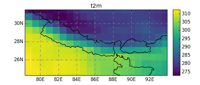
Currently, salem implements, the neirest neighbor (default), linear, and spline interpolation methods:

In [23]: dsr = ds.salem.transform(dse, interp='spline')

In [24]: dsr.t2m.mean(dim='time').salem.quick_map();

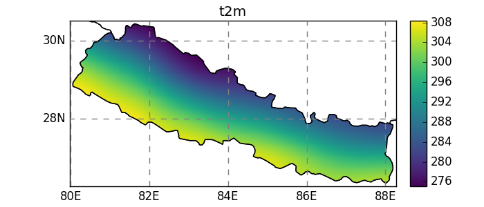
Subsetting data¶

In [25]: shdf = salem.read_shapefile(salem.get_demo_file('world_borders.shp'))

In [26]: shdf = shdf.loc[shdf['CNTRY_NAME'] == 'Nepal']

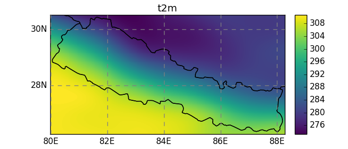
In [27]: dsr = dsr.salem.subset(shape=shdf, margin=10)

In [28]: dsr.t2m.mean(dim='time').salem.quick_map();

Regions of interest¶

In [29]: dsr = dsr.salem.roi(shape=shdf)

In [30]: dsr.t2m.mean(dim='time').salem.quick_map();