Map transformations
Most of the georeferencing machinery for gridded datasets is
handled by the Grid class: its capacity to handle
gridded datasets in a painless manner was one of the primary
motivations to develop Salem.
Grids
A point on earth can be defined unambiguously in two ways:
- DATUM (lon, lat, datum)
longitudes and latitudes are angular coordinates of a point on an ellipsoid (often called “datum”)
- PROJ (x, y, projection)
x (eastings) and y (northings) are cartesian coordinates of a point in a map projection (the unit of x, y is usually meter)
Salem adds a third coordinate reference system (crs) to this list:
- GRID (i, j, Grid)
on a structured grid, the (x, y) coordinates are distant of a constant (dx, dy) step. The (x, y) coordinates are therefore equivalent to a new reference frame (i, j) proportional to the projection’s (x, y) frame.
Transformations between datums and projections is handled by several tools in the python ecosystem, for example GDAL or the more lightweight pyproj, which is the tool used by Salem internally 1.
The concept of Grid added by Salem is useful when transforming data between two structured datasets, or from an unstructured dataset to a structured one.
- 1
Most datasets nowadays are defined in the WGS 84 datum, therefore the concepts of datum and projection are often interchangeable: (lon, lat) coordinates are equivalent to cartesian (x, y) coordinates in the plate carree projection.
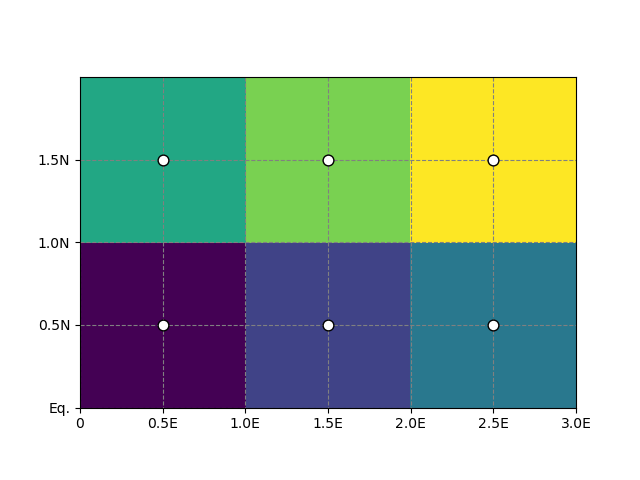
A Grid is defined by a projection, a reference point in
this projection, a grid spacing and a number of grid points:
In [1]: import numpy as np

In [2]: import salem

In [3]: from salem import wgs84

In [4]: grid = salem.Grid(nxny=(3, 2), dxdy=(1, 1), x0y0=(0.5, 0.5), proj=wgs84)

In [5]: x, y = grid.xy_coordinates

In [6]: x
Out[6]:
array([[0.5, 1.5, 2.5],
       [0.5, 1.5, 2.5]])

In [7]: y
Out[7]:
array([[0.5, 0.5, 0.5],
       [1.5, 1.5, 1.5]])
The default is to define the grids according to the pixels center point:
In [8]: smap = salem.Map(grid)

In [9]: smap.set_data(np.arange(6).reshape((2, 3)))

In [10]: lon, lat = grid.ll_coordinates

In [11]: smap.set_points(lon.flatten(), lat.flatten())

In [12]: smap.visualize(addcbar=False)
Out[12]:
{'imshow': <matplotlib.image.AxesImage at 0x7f9999ebdb80>,
 'contour': [],
 'contourf': []}
But with the pixel_ref keyword you can use another convention. For Salem,
the two conventions are identical:
In [13]: grid_c = salem.Grid(nxny=(3, 2), dxdy=(1, 1), x0y0=(0, 0),
   ....:                     proj=wgs84, pixel_ref='corner')
   ....:

In [14]: assert grid_c == grid
While it’s good to know how grids work, most of the time grids should be inferred directly from the data files (see also: Initializing the accessor):
In [15]: ds = salem.open_xr_dataset(salem.get_demo_file('himalaya.tif'))

In [16]: grid = ds.salem.grid

In [17]: grid.proj.srs
Out[17]: '+proj=longlat +datum=WGS84 +no_defs'

In [18]: grid.extent
Out[18]: [78.31251347311601, 93.9375142881032, 24.237496572347762, 31.545830286884]
Grids come with several convenience functions, for example for transforming points onto the grid coordinates:
In [19]: grid.transform(85, 27, crs=salem.wgs84)
Out[19]: (801.9983413684238, 544.9996059728029)
Or for reprojecting structured data as explained below.
Reprojecting data
Interpolation
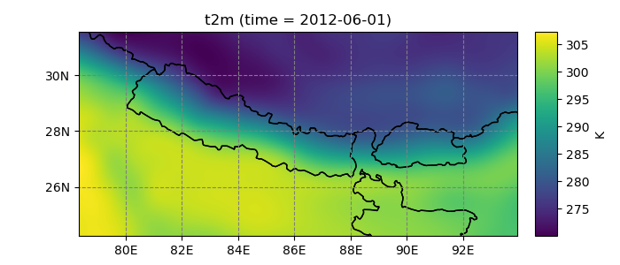
The standard way to reproject a gridded dataset into another one is to use the
transform() method:
In [20]: dse = salem.open_xr_dataset(salem.get_demo_file('era_interim_tibet.nc'))

In [21]: t2_era_reproj = ds.salem.transform(dse.t2m.isel(time=0))

In [22]: t2_era_reproj.salem.quick_map();

This is the recommended way if the output grid (in this case, a high resolution
lon-lat grid) is of similar or finer resolution than the input grid (in this
case, reanalysis data at 0.75°). As of v0.2, three interpolation methods are
available in Salem: nearest (default), linear, or spline:
In [23]: t2_era_reproj = ds.salem.transform(dse.t2m.isel(time=0), interp='spline')

In [24]: t2_era_reproj.salem.quick_map();
Internally, Salem uses pyproj for the coordinates transformation and scipy’s interpolation methods for the resampling. Note that reprojecting data can be computationally and memory expensive: it is generally recommended to reproject your data at the end of the processing chain if possible.
The transform() method returns an object of
the same structure as the input. The only differences are the coordinates and
the grid, which are those of the arrival grid:
In [25]: dst = ds.salem.transform(dse)

In [26]: dst
Out[26]:
<xarray.Dataset>
Dimensions:  (time: 4, x: 1875, y: 877)
Coordinates:
  * time     (time) datetime64[ns] 2012-06-01 ... 2012-06-01T18:00:00
  * x        (x) float64 78.32 78.33 78.33 78.34 ... 93.91 93.92 93.93 93.93
  * y        (y) float64 31.54 31.53 31.52 31.52 ... 24.27 24.26 24.25 24.24
Data variables:
    t2m      (time, y, x) float32 278.6 278.6 278.6 278.6 ... 296.2 296.2 296.2
Attributes:
    pyproj_srs:  +proj=longlat +datum=WGS84 +no_defs

In [27]: dst.salem.grid == ds.salem.grid
Out[27]: True
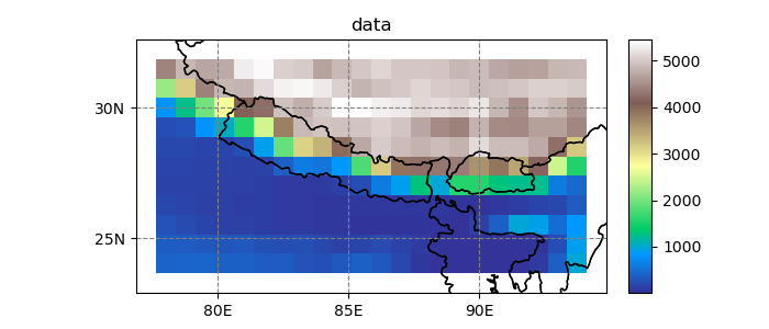
Aggregation
If you need to resample higher resolution data onto a coarser grid,
lookup_transform() may be the way to go. This
method gets its name from the “lookup table” it uses internally to store
the information needed for the resampling: for each
grid point in the coarser dataset, the lookup table stores the coordinates
of the high-resolution grid located below.
The default resampling method is to average all these points:
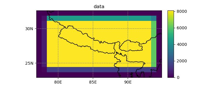
In [28]: dse = dse.salem.subset(corners=((77, 23), (94.5, 32.5)))

In [29]: dsl = dse.salem.lookup_transform(ds)

In [30]: dsl.data.salem.quick_map(cmap='terrain');
But any aggregation method is available, for example np.std, or len if
you want to know the number of high resolution pixels found below a coarse
grid point:
In [31]: dsl = dse.salem.lookup_transform(ds, method=len)

In [32]: dsl.data.salem.quick_map();