WRF tools
Let’s open a WRF model output file with xarray first:
In [1]: import xarray as xr

In [2]: from salem.utils import get_demo_file

In [3]: ds = xr.open_dataset(get_demo_file('wrfout_d01.nc'))
WRF files are a bit messy:
In [4]: ds
Out[4]:
<xarray.Dataset>
Dimensions:           (Time: 3, bottom_top: 27, bottom_top_stag: 28, south_north: 150, south_north_stag: 151, west_east: 150, west_east_stag: 151)
Coordinates:
    XLONG             (Time, south_north, west_east) float32 70.7231 70.9749 ...
    XLONG_U           (Time, south_north, west_east_stag) float32 70.5974 ...
    XLAT_U            (Time, south_north, west_east_stag) float32 7.76865 ...
    XLAT_V            (Time, south_north_stag, west_east) float32 7.66444 ...
    XLONG_V           (Time, south_north_stag, west_east) float32 70.7436 ...
    XLAT              (Time, south_north, west_east) float32 7.78907 7.82944 ...
  * Time              (Time) int64 0 1 2
  * south_north       (south_north) int64 0 1 2 3 4 5 6 7 8 9 10 11 12 13 14 ...
  * west_east         (west_east) int64 0 1 2 3 4 5 6 7 8 9 10 11 12 13 14 ...
  * bottom_top        (bottom_top) int64 0 1 2 3 4 5 6 7 8 9 10 11 12 13 14 ...
  * west_east_stag    (west_east_stag) int64 0 1 2 3 4 5 6 7 8 9 10 11 12 13 ...
  * south_north_stag  (south_north_stag) int64 0 1 2 3 4 5 6 7 8 9 10 11 12 ...
  * bottom_top_stag   (bottom_top_stag) int64 0 1 2 3 4 5 6 7 8 9 10 11 12 ...
Data variables:
    Times             (Time) |S19 '2008-10-26_12:00:00' ...
    T2                (Time, south_north, west_east) float32 301.977 302.008 ...
    RAINC             (Time, south_north, west_east) float32 0.0 0.0 0.0 0.0 ...
    RAINNC            (Time, south_north, west_east) float32 0.0 0.0 0.0 0.0 ...
    U                 (Time, bottom_top, south_north, west_east_stag) float32 1.59375 ...
    V                 (Time, bottom_top, south_north_stag, west_east) float32 -2.07031 ...
    PH                (Time, bottom_top_stag, south_north, west_east) float32 0.0 ...
    PHB               (Time, bottom_top_stag, south_north, west_east) float32 0.0 ...
Attributes:
    note: Global attrs removed.
WRF files aren’t exactly CF compliant: you’ll need a special parser for the timestamp, the coordinate names are a bit exotic and do not correspond to the dimension names, they contain so-called staggered variables (and their correponding coordinates), etc.
Salem defines a special parser for these files:
In [5]: import salem

In [6]: ds = salem.open_wrf_dataset(get_demo_file('wrfout_d01.nc'))
This parser greatly simplifies the file structure:
In [7]: ds
Out[7]:
<xarray.Dataset>
Dimensions:       (bottom_top: 27, south_north: 150, time: 3, west_east: 150)
Coordinates:
    lon           (time, south_north, west_east) float32 70.7231 70.9749 ...
    lat           (time, south_north, west_east) float32 7.78907 7.82944 ...
  * time          (time) datetime64[ns] 2008-10-26T12:00:00 ...
  * south_north   (south_north) float64 -2.235e+06 -2.205e+06 -2.175e+06 ...
  * west_east     (west_east) float64 -2.235e+06 -2.205e+06 -2.175e+06 ...
  * bottom_top    (bottom_top) int64 0 1 2 3 4 5 6 7 8 9 10 11 12 13 14 15 ...
Data variables:
    T2            (time, south_north, west_east) float32 301.977 302.008 ...
    RAINC         (time, south_north, west_east) float32 0.0 0.0 0.0 0.0 0.0 ...
    RAINNC        (time, south_north, west_east) float32 0.0 0.0 0.0 0.0 0.0 ...
    U             (time, bottom_top, south_north, west_east) float32 1.73438 ...
    V             (time, bottom_top, south_north, west_east) float32 -2.125 ...
    PH            (time, bottom_top, south_north, west_east) float32 18.7031 ...
    PHB           (time, bottom_top, south_north, west_east) float32 277.504 ...
    T2C           (time, south_north, west_east) float32 28.8266 28.8578 ...
    PRCP          (time, south_north, west_east) float32 nan nan nan nan nan ...
    GEOPOTENTIAL  (time, bottom_top, south_north, west_east) float32 296.207 ...
    PRCP_NC       (time, south_north, west_east) float32 nan nan nan nan nan ...
    PRCP_C        (time, south_north, west_east) float32 nan nan nan nan nan ...
Attributes:
    note: Global attrs removed.
Note that some dimensions / coordinates have been renamed, new variables have been defined, and the staggered dimensions have disappeared.
Diagnostic variables
Salem adds a layer between xarray and the underlying NetCDF file. This layer computes new variables “on the fly” or, in the case of staggered variables, “unstaggers” them:
In [8]: ds.U
Out[8]:
<xarray.DataArray 'U' (time: 3, bottom_top: 27, south_north: 150, west_east: 150)>
[1822500 values with dtype=float32]
Coordinates:
    lon          (time, south_north, west_east) float32 70.7231 70.9749 ...
    lat          (time, south_north, west_east) float32 7.78907 7.82944 ...
  * time         (time) datetime64[ns] 2008-10-26T12:00:00 ...
  * south_north  (south_north) float64 -2.235e+06 -2.205e+06 -2.175e+06 ...
  * west_east    (west_east) float64 -2.235e+06 -2.205e+06 -2.175e+06 ...
  * bottom_top   (bottom_top) int64 0 1 2 3 4 5 6 7 8 9 10 11 12 13 14 15 16 ...
Attributes:
    FieldType: 104
    MemoryOrder: XYZ
    description: x-wind component
    units: m s-1
    stagger: X
    pyproj_srs: +units=m +proj=lcc +lat_1=29.0400009155 +lat_2=29.0400009155 +lat_0=29.0399971008 +lon_0=89.8000030518 +x_0=0 +y_0=0 +a=6370000 +b=6370000
This computation is done only on demand (just like a normal NetCDF variable), this new layer is therefore relatively cheap.
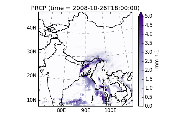
In addition to unstaggering, Salem adds a number of “diagnostic” variables to the dataset. Some are convenient (like T2C, temperature in Celsius instead of Kelvins), but others are more complex (e.g. SLP for sea-level pressure, or PRCP which computes step-wize total precipitation out of the accumulated fields). For a list of diagnostic variables (and TODOs!), refer to GH18.
In [9]: ds.PRCP.isel(time=-1).salem.quick_map(cmap='Purples', vmax=5)
Out[9]: <salem.graphics.Map at 0x7f028a580250>
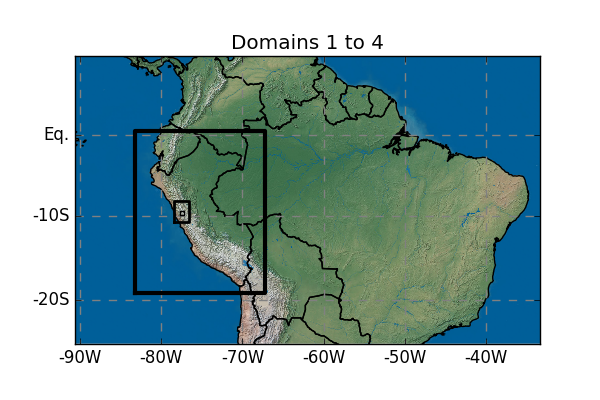
Geogrid simulator
Salem provides a small tool which comes handy when defining new WRF domains. It parses the WPS configuration file (namelist.wps) and generates the grids and maps corresponding to each domain.
geogrid_simulator() will search for the &geogrid section of the file and parse it:
In [10]: fpath = get_demo_file('namelist_mercator.wps')

In [11]: with open(fpath, 'r') as f:  # this is just to show the file
   ....:     print(f.read())
   ....:
&geogrid
 parent_id         =   1, 1, 2, 3,
 parent_grid_ratio =   1, 3, 5, 5,
 i_parent_start    =   1, 28, 54, 40,
 j_parent_start    =   1, 24, 97, 50,
 e_we              =  211, 178, 101, 136,
 e_sn              =  131, 220, 141, 136,
 dx = 30000,
 dy = 30000,
 map_proj = 'mercator',
 ref_lat   =  -8.0,
 ref_lon   =  -62.0,
 truelat1  =  -8.0,
/


In [12]: from salem import geogrid_simulator

In [13]: g, maps = geogrid_simulator(fpath)

In [14]: maps[0].set_rgb(natural_earth='lr')  # add a background image
Downloading Natural Earth lr...

In [15]: maps[0].visualize(title='Domains 1 to 4')