Examples
Subsetting and selecting data
Let’s open a WRF model output file:
In [1]: import salem

In [2]: from salem.utils import get_demo_file

In [3]: ds = salem.open_xr_dataset(get_demo_file('wrfout_d01.nc'))
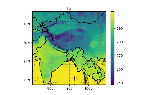
Let’s take a time slice of the variable T2 for a start:
In [4]: t2 = ds.T2.isel(Time=2)

In [5]: t2.salem.quick_map()
Out[5]: <salem.graphics.Map at 0x7f491ebded68>
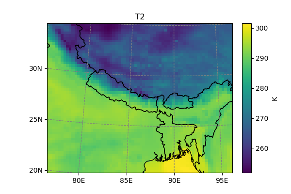
Although we are on a Lambert Conformal projection, it’s possible to subset the file using longitudes and latitudes:
In [6]: t2_sub = t2.salem.subset(corners=((77., 20.), (97., 35.)), crs=salem.wgs84)

In [7]: t2_sub.salem.quick_map()
Out[7]: <salem.graphics.Map at 0x7f491cf3de10>
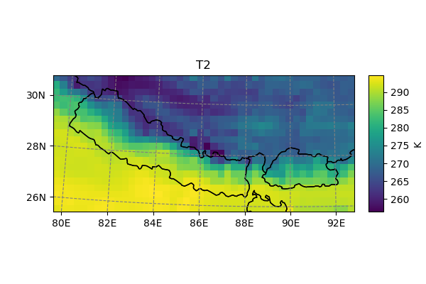
It’s also possible to use geometries or shapefiles to subset your data:
In [8]: shdf = salem.read_shapefile(get_demo_file('world_borders.shp'))

In [9]: shdf = shdf.loc[shdf['CNTRY_NAME'].isin(['Nepal', 'Bhutan'])]  # GeoPandas' GeoDataFrame

In [10]: t2_sub = t2_sub.salem.subset(shape=shdf, margin=2)  # add 2 grid points

In [11]: t2_sub.salem.quick_map()
Out[11]: <salem.graphics.Map at 0x7f491c659748>
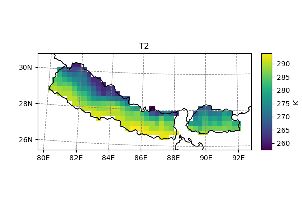
Based on the same principle, one can mask out the useless grid points:
In [12]: t2_roi = t2_sub.salem.roi(shape=shdf)

In [13]: t2_roi.salem.quick_map()
Out[13]: <salem.graphics.Map at 0x7f491ed47400>
Plotting
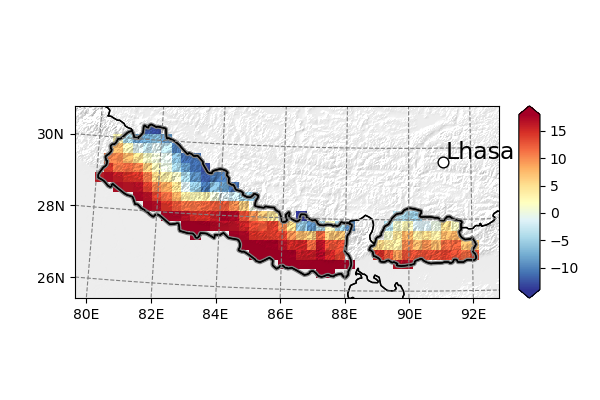
Maps can be pimped with topographical shading, points of interest, and more:
In [14]: smap = t2_roi.salem.get_map(data=t2_roi-273.15, cmap='RdYlBu_r', vmin=-14, vmax=18)

In [15]: _ = smap.set_topography(get_demo_file('himalaya.tif'))

In [16]: smap.set_shapefile(shape=shdf, color='grey', linewidth=3)

In [17]: smap.set_points(91.1, 29.6)

In [18]: smap.set_text(91.2, 29.7, 'Lhasa', fontsize=17)

In [19]: smap.visualize()
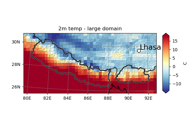
Maps are persistent, which is useful when you have many plots to do. Plotting further data on them is possible, as long as the geolocalisation information is shipped with the data (in that case, the DataArray’s attributes are lost in the conversion from Kelvins to degrees Celsius so we have to set it explicitly):
In [20]: smap.set_data(ds.T2.isel(Time=1)-273.15, crs=ds.salem.grid)

In [21]: smap.visualize(title='2m temp - large domain', cbar_title='C')
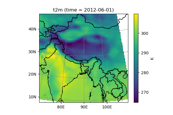
Reprojecting data
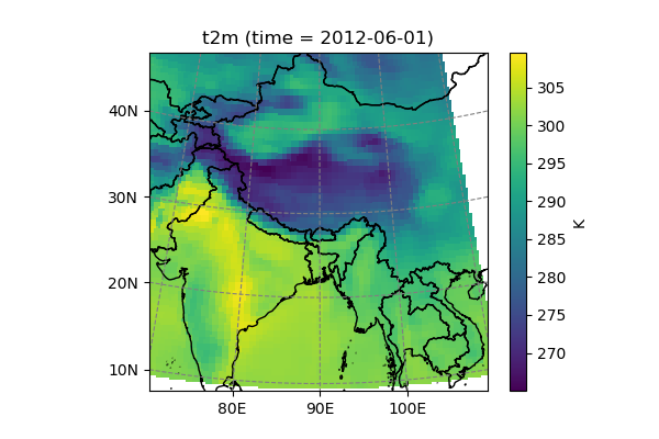
Salem can also transform data from one grid to another:
In [22]: dse = salem.open_xr_dataset(get_demo_file('era_interim_tibet.nc'))

In [23]: t2_era_reproj = ds.salem.transform(dse.t2m)

In [24]: assert t2_era_reproj.salem.grid == ds.salem.grid

In [25]: t2_era_reproj.isel(time=0).salem.quick_map()
Out[25]: <salem.graphics.Map at 0x7f491d3e5048>
In [26]: t2_era_reproj = ds.salem.transform(dse.t2m, interp='spline')

In [27]: t2_era_reproj.isel(time=0).salem.quick_map()
Out[27]: <salem.graphics.Map at 0x7f491ee83128>