WRF tools
Let’s open a WRF model output file with xarray first:
In [1]: import xarray as xr

In [2]: from salem.utils import get_demo_file

In [3]: ds = xr.open_dataset(get_demo_file('wrfout_d01.nc'))
WRF files are a bit messy:
In [4]: ds
Out[4]:
<xarray.Dataset>
Dimensions:  (Time: 3, bottom_top: 27, bottom_top_stag: 28, south_north: 150, south_north_stag: 151, west_east: 150, west_east_stag: 151)
Coordinates:
    XLONG    (Time, south_north, west_east) float32 ...
    XLONG_U  (Time, south_north, west_east_stag) float32 ...
    XLAT_U   (Time, south_north, west_east_stag) float32 ...
    XLAT_V   (Time, south_north_stag, west_east) float32 ...
    XLONG_V  (Time, south_north_stag, west_east) float32 ...
    XLAT     (Time, south_north, west_east) float32 ...
Dimensions without coordinates: Time, bottom_top, bottom_top_stag, south_north, south_north_stag, west_east, west_east_stag
Data variables:
    Times    (Time) |S19 ...
    T2       (Time, south_north, west_east) float32 ...
    RAINC    (Time, south_north, west_east) float32 ...
    RAINNC   (Time, south_north, west_east) float32 ...
    U        (Time, bottom_top, south_north, west_east_stag) float32 ...
    V        (Time, bottom_top, south_north_stag, west_east) float32 ...
    PH       (Time, bottom_top_stag, south_north, west_east) float32 ...
    PHB      (Time, bottom_top_stag, south_north, west_east) float32 ...
Attributes:
    note:     Global attrs removed.
WRF files aren’t exactly CF compliant: you’ll need a special parser for the timestamp, the coordinate names are a bit exotic and do not correspond to the dimension names, they contain so-called staggered variables (and their correponding coordinates), etc.
Salem defines a special parser for these files:
In [5]: import salem

In [6]: ds = salem.open_wrf_dataset(get_demo_file('wrfout_d01.nc'))
This parser greatly simplifies the file structure:
In [7]: ds
Out[7]:
<xarray.Dataset>
Dimensions:       (bottom_top: 27, south_north: 150, time: 3, west_east: 150)
Coordinates:
    lon           (south_north, west_east) float32 70.723145 70.97485 ...
    lat           (south_north, west_east) float32 7.78907 7.8294373 ...
  * time          (time) datetime64[ns] 2008-10-26T12:00:00 ...
  * west_east     (west_east) float64 -2.235e+06 -2.205e+06 -2.175e+06 ...
  * south_north   (south_north) float64 -2.235e+06 -2.205e+06 -2.175e+06 ...
Dimensions without coordinates: bottom_top
Data variables:
    T2            (time, south_north, west_east) float32 ...
    RAINC         (time, south_north, west_east) float32 ...
    RAINNC        (time, south_north, west_east) float32 ...
    U             (time, bottom_top, south_north, west_east) float32 ...
    V             (time, bottom_top, south_north, west_east) float32 ...
    PH            (time, bottom_top, south_north, west_east) float32 ...
    PHB           (time, bottom_top, south_north, west_east) float32 ...
    WS            (time, bottom_top, south_north, west_east) float32 ...
    T2C           (time, south_north, west_east) float32 ...
    GEOPOTENTIAL  (time, bottom_top, south_north, west_east) float32 ...
    Z             (time, bottom_top, south_north, west_east) float32 ...
    PRCP          (time, south_north, west_east) float32 ...
    PRCP_NC       (time, south_north, west_east) float32 ...
    PRCP_C        (time, south_north, west_east) float32 ...
Attributes:
    pyproj_srs:  +units=m +proj=lcc +lat_1=29.040000915527344 +lat_2=29.04000...
    note:        Global attrs removed.
Note that some dimensions / coordinates have been renamed, new variables have been defined, and the staggered dimensions have disappeared.
Diagnostic variables
Salem adds a layer between xarray and the underlying NetCDF file. This layer computes new variables “on the fly” or, in the case of staggered variables, “unstaggers” them:
In [8]: ds.U
Out[8]:
<xarray.DataArray 'U' (time: 3, bottom_top: 27, south_north: 150, west_east: 150)>
[1822500 values with dtype=float32]
Coordinates:
    lon          (south_north, west_east) float32 70.723145 70.97485 ...
    lat          (south_north, west_east) float32 7.78907 7.8294373 ...
  * time         (time) datetime64[ns] 2008-10-26T12:00:00 ...
  * west_east    (west_east) float64 -2.235e+06 -2.205e+06 -2.175e+06 ...
  * south_north  (south_north) float64 -2.235e+06 -2.205e+06 -2.175e+06 ...
Dimensions without coordinates: bottom_top
Attributes:
    FieldType:    104
    MemoryOrder:  XYZ
    description:  x-wind component
    units:        m s-1
    stagger:      X
    pyproj_srs:   +units=m +proj=lcc +lat_1=29.040000915527344 +lat_2=29.0400...
This computation is done only on demand (just like a normal NetCDF variable), this new layer is therefore relatively cheap.
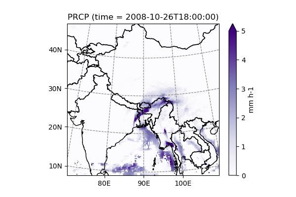
In addition to unstaggering, Salem adds a number of “diagnostic” variables
to the dataset. Some are convenient (like T2C, temperature in Celsius
instead of Kelvins), but others are more complex (e.g. SLP for sea-level
pressure, or PRCP which computes step-wize total precipitation out of the
accumulated fields). For a list of diagnostic variables (and TODOs!), refer to
GH18.
In [9]: ds.PRCP.isel(time=-1).salem.quick_map(cmap='Purples', vmax=5)
Out[9]: <salem.graphics.Map at 0x7f491ec7f550>
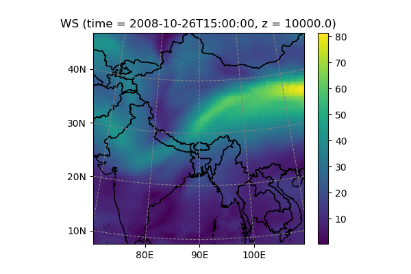
Vertical interpolation
The WRF vertical coordinates are eta-levels, which is not a very practical
coordinate for analysis or plotting. With the functions
wrf_zlevel() and
wrf_plevel() it is possible to interpolate the 3d
data at either altitude or pressure levels:
In [10]: ws_h = ds.isel(time=1).salem.wrf_zlevel('WS', levels=10000.)

In [11]: ws_h.salem.quick_map();
Note that currently, the interpolation is quite slow, see GH25. It’s probably wise to do it on single time slices or aggregated data, rather than huge data cubes.
Open multiple files
It is possible to open multiple WRF files at different time steps with
open_mf_wrf_dataset(), which works like xarray’s
open_mfdataset . The only drawback of having multiple WRF time slices is
that “de-accumulated” variables such as PRCP won’t be available.
For this purpose, you might want to use the deacc()
method.
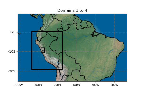
Geogrid simulator
Salem provides a small tool which comes handy when defining new WRF domains. It parses the WPS configuration file (namelist.wps) and generates the grids and maps corresponding to each domain.
geogrid_simulator() will search for the &geogrid section of the
file and parse it:
In [12]: fpath = get_demo_file('namelist_mercator.wps')

In [13]: with open(fpath, 'r') as f:  # this is just to show the file
   ....:     print(f.read())
   ....:
&geogrid
 parent_id         =   1, 1, 2, 3,
 parent_grid_ratio =   1, 3, 5, 5,
 i_parent_start    =   1, 28, 54, 40,
 j_parent_start    =   1, 24, 97, 50,
 e_we              =  211, 178, 101, 136,
 e_sn              =  131, 220, 141, 136,
 dx = 30000,
 dy = 30000,
 map_proj = 'mercator',
 ref_lat   =  -8.0,
 ref_lon   =  -62.0,
 truelat1  =  -8.0,
/


In [14]: from salem import geogrid_simulator

In [15]: g, maps = geogrid_simulator(fpath)

In [16]: maps[0].set_rgb(natural_earth='lr')  # add a background image

In [17]: maps[0].visualize(title='Domains 1 to 4')