Plot on a google map background

Google static maps API

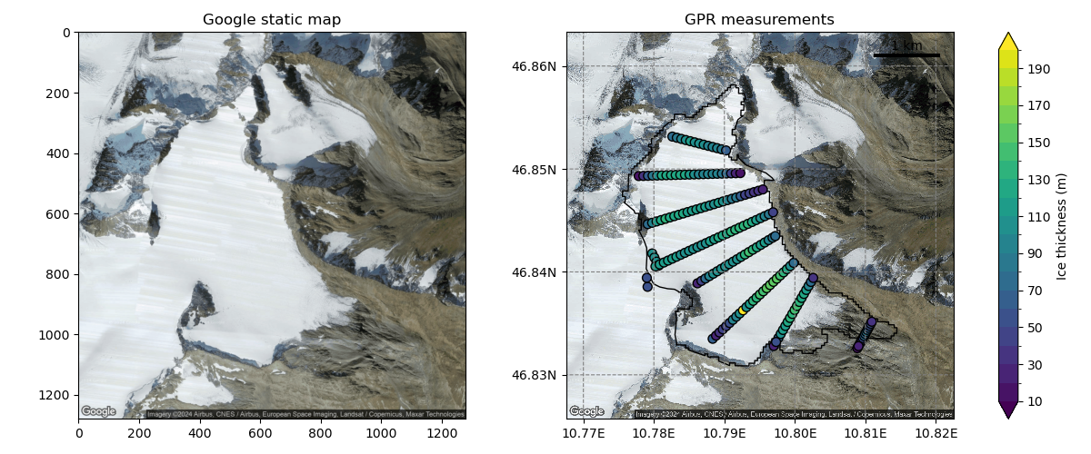
In this script, we use motionless to download an image from the google static map API and plot it on a Map. We then add information to the map such as a glacier outline (from the RGI), and ground penetrating radar measurements (GPR, from the GlaThiDa database).

The GPR measurements were realized in 1997, the glacier outlines are from 2003, and the map background is from 2016. This illustrates the retreat of the Kesselwandferner glacier.

/home/docs/checkouts/readthedocs.org/user_builds/salem/conda/stable/lib/python3.12/site-packages/pyproj/utils.py:135: FutureWarning: Calling float on a single element Series is deprecated and will raise a TypeError in the future. Use float(ser.iloc[0]) instead
  xxx = array("d", xxx)

import numpy as np
import pandas as pd
import salem
from salem import get_demo_file, DataLevels, GoogleVisibleMap, Map
import matplotlib.pyplot as plt

# prepare the figure
f, (ax1, ax2) = plt.subplots(1, 2, figsize=(12, 5))

# read the shapefile and use its extent to define a ideally sized map
shp = salem.read_shapefile(get_demo_file('rgi_kesselwand.shp'))
# For this to work you'll need to use an API key and set it
# here with key='YOUR_API_KEY' or set it as an
# environment variable called STATIC_MAP_API_KEY
g = GoogleVisibleMap(x=[shp.min_x, shp.max_x], y=[shp.min_y, shp.max_y],
                     scale=2,  # scale is for more details
                     maptype='satellite')  # try out also: 'terrain'

# the google static image is a standard rgb image
ggl_img = g.get_vardata()
ax1.imshow(ggl_img)
ax1.set_title('Google static map')

# make a map of the same size as the image (no country borders)
sm = Map(g.grid, factor=1, countries=False)
sm.set_shapefile(shp)  # add the glacier outlines
sm.set_rgb(ggl_img)  # add the background rgb image
sm.set_scale_bar(location=(0.88, 0.94))  # add scale
sm.visualize(ax=ax2)  # plot it
ax2.set_title('GPR measurements')

# read the point GPR data and add them to the plot
df = pd.read_csv(get_demo_file('gtd_ttt_kesselwand.csv'))
dl = DataLevels(df.THICKNESS, levels=np.arange(10, 201, 10), extend='both')
x, y = sm.grid.transform(df.POINT_LON.values, df.POINT_LAT.values)
ax2.scatter(x, y, color=dl.to_rgb(), s=50, edgecolors='k', linewidths=1)
dl.append_colorbar(ax2, label='Ice thickness (m)')

# make it nice
plt.tight_layout()
plt.show()